Implementing streaming features comes with two main challenges:

1. Serving performance: freshness and latency, especially for features that might perform complex aggregations and transformations over varying window sizes.
2. Point-in-time-correct (PITC) backfills: Producing historical values accurate as of observation timestamps without forcing the user to wait for logs or asking them to compute historical feature values in a separate job.

There are a range of solutions on the market that take various architectural approaches, each with their own considerations:

1. Bring-your-own-compute architecture: The onus of writing and maintaining streaming jobs and batch jobs that produce historical values is put on the user.
   1. Writing a streaming job that scalably maintains state, correctly handles tail-eviction, combines batch processing for window-seeding and correction is very complex. MLEs should be empowered to focus on building features and models, not writing streaming pipelines.
   2. Users must still write the streaming job described above and a batch job that reconstructs that same state for historical points in time. Both must be kept in sync as the user makes changes or adds features to their models. As you scale to more features, inconsistency becomes inevitable.
2. Batch compute-based architectures, i.e. Snowflake: claim to achieve streaming by having streaming ingestion plus some concept of incremental computation or more frequent batches.
   1. Many useful ML features like windowed aggregations cannot be produced via incrementalizable queries, so as you increase the frequency of your batches, you increase cost substantially.
   2. Freshness is far worse than a true streaming system, especially when considered alongside point (a) above. This is a deal-breaker for many use cases.
3. Naive streaming compute-based architectures, i.e. Databricks Declarative Features (in Beta as of publication date): Backfills and online pipelines are driven by the same declarative feature definition, but streaming state is maintained in a naive manner.
   1. This architecture solves the online/offline consistency challenge by unifying computation for backfills and serving.
   2. Performance becomes a challenge at scale, forcing users to choose between freshness and latency.
4. Scalable streaming compute-based architecture, i.e. Zipline: Backfills and online pipelines are driven by the same declarative feature definition, and the streaming job implementation compresses state to constant size relative to window length while maintaining freshness.
   1. This architecture solves the online/offline consistency challenge by unifying computation for backfills and serving, and does so cheaply by leveraging partial-aggregate caching to achieve compute-reuse across jobs.
   2. Removes the tradeoff between freshness and performance at scale, allowing users to implement flexible aggregations over arbitrarily large windows without latency or stability degradation.

Example / Requirements

Throughout this article we’ll work with a simple feature definition: `average transaction amount by user in the last 7 days.`

Requirements:

• Freshness: Online values are served with ~1s freshness (events come in via Kafka/Kinesis/Pubsub).
• Tail accuracy: fetching a value correctly excludes events outside of the tail of the window (`now - 7days`)
• Bootstrapping: Feature data can be backfilled for the last ~1 year using historical raw transaction data in the warehouse immediately upon defining the feature. Does not require the user to run a separate historical ETL job, or wait for logged values.
• Consistency: backfills and online values have consistency guarantees for arbitrary observation (key, timestamp) pairs that can be specified by the user at backfill-time.
• Scale: Need to support tens of thousands of features across a range of common workloads, including search ranking which needs those features across thousands of candidates at many thousand RPS with very tight latency budgets (<10ms).

Technical Deep Dive

Next we’ll dig into the various architectures and how they perform against the above requirements.

Zipline’s Approach

Zipline offers a declarative feature definition API that would look something like the below for this example:

Aggregation(
  input_column="transaction_amt",
  operation=Operation.AVERAGE,
  windows=["7d"]
)

From this single definition, a user can:

• Serve this feature in real-time with <10ms latency
• Backfill this feature for any arbitrary “observation spine” and get PITC feature values for those observations
  • Values that are consistent with what would have been served online for those observation timestamps.

Online

After defining the feature (as shown above), all the user needs to do is call zipline hub run-adhoc

Then Zipline automates the following batch and streaming jobs, and creation of fetcher endpoint:

Batch upload job:

The batch upload job serves the following role in the streaming architecture:

1. Seed initial values: streaming topics don’t always hold sufficient data to compute the entire window, and even if they did you wouldn’t necessarily want to perform large scale batch aggregation within your streaming engine. By populating the streaming state with history from batch, the streaming job itself only needs to start as-of the effective upload cutoff time.
2. Compress window state: This is a critical piece of the architecture that enables constant latency with arbitrary window sizes. See CollapsedIR below for more details.
3. Batch correction: data issues or interruptions to streaming jobs shouldn’t cause persistent data issues online. Batch jobs can reset state reliably on a scheduled cadence.

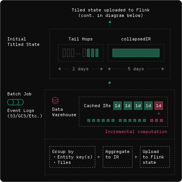
*Note on Intermediate Representation (IR): In this case, since we’re performing an AVERAGE, the IR would be a (sum, count) pair. A key point is that IRs turn aggregations into composable values that can be combined across various time windows to produce correct final results. Zipline leverages this to compress state from raw events to a single IR per key in a given time range.*

The batch job produces the following:

1. CollapsedIR: A single IR for the middle of the window, excluding the last 2 days. I.e. for a 7 day window, this is 5 days aggregated value. For 30 days it would be 28 days, etc.
2. tailHops: 1-hour bucketed IRs for the tailing 2 days of the window. These are only created for windowed aggregations that require tail accuracy (all-time agg only needs a CollapsedIR which covers the entire range). At read time, the Fetcher includes only the hops required to correctly compute the window (i.e. cutoff at `now - 7d`), thus achieving tail accuracy.

Streaming Job:

The streaming job is responsible for updating the state and the final values being served out of the KV store when new events enter or leave the tail of the window.

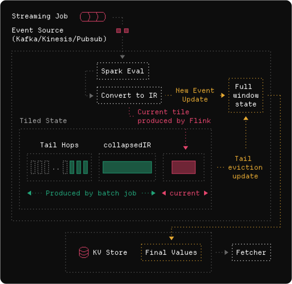
*Note on Spark Eval: Zipline allows users to define arbitrary column-level SQL transformations as part of the streaming transformation. For example, in the feature definition above, a user could define as input_column="transaction_amt / 100" or any other Spark-SQL transformation. The Zipline engine applies these Spark projections within the Flink pipelines and at backfill time to ensure consistency.*

The streaming job achieves this by implementing the following:

1. On new event: Converts the event to an IR then combines it with the record for that key in the full window state, keeping that value up to date.
2. On tail eviction (tail hop falling out of the window): Combines remaining valid tail hops, the collapsedIR, and the head tile into a single value per key and updates necessary records in full window state.
3. On either of the above: Converts IR to finalized value, i.e. applies the finalize operation to convert (sum, count) pair into an average by doing sum / count, then writes the key/value pair to the KV store.

Result: <10ms feature serving with any window size. Increasing window size does not increase the size of streaming state, or size of payload that is fetched and returned at read time. It only increases the workload of the batch process, and only on the first run thanks to incremental computation that can be achieved by producing and caching IRs of partial aggregates, to be covered in further detail in a future post.

Offline

First off, why are we talking about backfills in a post about streaming features? Streaming is for online serving, backfills is a separate batch process, right?

To use a streaming feature in production you need to backfill it for model training, and that leaves you with one of three options:

1. Write your streaming pipeline and log values for training (log-and-wait). The issue is many models need months or years of data to train on, and that’s too long to wait.
2. Write your streaming logic in one place and different ETL for your training data generation. Now you have dual pipelines that must be kept in sync, and inconsistencies create difficult to debug issues in production.
3. Use a unified engine like Zipline to power both training and serving, guaranteeing consistency and fast backfills.

To run a backfill in zipline, all the user needs to do is define the spine of their backfill, add the features that they want via the Join API, then call zipline hub backfill

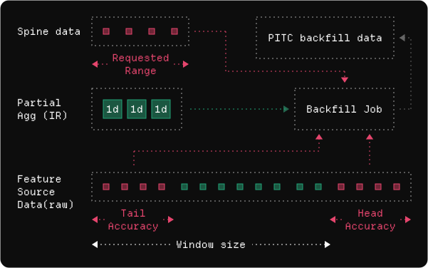
Zipline does this by using the SawtoothAggregator that mimics the hopping window accuracy produced by the tiled streaming architecture that serves the online flow.

The spine is responsible for producing the primary keys and timestamps at which a backfill should be accurate as-of (i.e. prediction times), and Zipline’s engine produces historical values consistent with what would have been served online at those points in time.

There are many more optimizations within Zipline backfills, including:

• Surgical recomputation when you change one or a few out of many features in a table
• Feature sharing across same/different spines with compute reuse
• Safe and efficient experimentation using versioning and branching

Those topics and many more are reserved for a different blog post that we hope to publish soon.

Bring-Your-Own-Compute

This architecture is focused only on storing and serving feature values, putting the onus of building and maintaining streaming and batch computation pipelines on the user.

The issue with this, as outlined below are twofold:

1. The complexity of building scalable streaming pipelines (see the Zipline architecture above)
2. Generating point-in-time-correct backfills requires building a secondary batch pipeline (introduces inconsistency) or relying on logged values (too slow).

More details below.

Online

To serve a streaming feature in a bring-your-own-compute architecture, the user has to build and operate the full computation stack themselves.

There are many implementation choices here: raw-event append, timer-driven stateful streaming, tiled aggregation schemes, etc.

This architecture inherently pushes substantial complexity onto the user. DS and MLE should be focused on authoring features, training models, and running experiments, not complex streaming pipelines.

Offline

On the offline side, BYOC architectures usually claim to solve the online/offline problem with an as-of join. However, this is far from a true solution. The user still needs to write a job that populates historical values that flow into the as-of join.

Now this batch job and the streaming job must implement the same:

• window definition
• aggregation semantics
• tail-eviction logic
• late-data behavior
• Read-time transformation logic
• Etc.

So in practice, BYOC leaves the user with a bad option and a worse one:

1. Dual pipelines: Build one pipeline for online serving and another for historical backfills, then try to keep them perfectly in sync as you add more features or try to make changes to existing ones.
2. Log-and-wait: Depend on previously served values, which limits how far back you can train and makes experimentation painful. Furthermore, a new spine with different observation timestamps would need to restart the waiting period. This is simply too slow of an iteration loop for any meaningful use case.

Batch Compute-based architecture (i.e. Snowflake)

This is an interesting one because this architecture essentially doesn’t even try when it comes to streaming.

Online Flow

In this architecture, “streaming” is really continuous ingestion plus scheduled recomputation. The user defines a feature as a query over raw data, and the platform materializes the results into a feature table on a refresh cadence using a system like Snowflake-managed feature view backed by a dynamic table.

Snowflake explicitly says managed feature views are refreshed on a schedule you specify, and that dynamic tables use incremental refresh when possible but fall back to full refresh when incremental refresh is unsupported or inefficient. “The feature table is automatically refreshed from raw data by Snowflake on a schedule you specify” (link).

This is where the drawbacks from the intro show up:

• Freshness is bounded by refresh frequency. Even with continuous ingestion, online values only change when the dynamic table refreshes, and Snowflake only guarantees a target lag, not true event-by-event updates.
• Windowed aggregations become expensive at high freshness. Most aggregations that are useful for ML are not incrementalizable, so as refreshes become more frequent, recomputation cost rises sharply; Snowflake’s docs are explicit that if incremental refresh is unsupported or inefficient, it will choose full refresh instead. In this example, each batch would scan and aggregate 7 days of data.

Offline Flow

Because this architecture is fundamentally batch-based, the same pipeline can be used both to compute historical feature values and to power the “online” path, which is really just a scheduled job that refreshes the latest values. That makes online/offline consistency a much easier problem than in bring-your-own-compute systems. You can run the same batch computation over history and join the resulting values to an observation spine using standard as-of semantics. However, that’s only because this architecture really doesn’t implement streaming.

Naive Streaming-based architecture (i.e. Databricks declarative feature)

The Databricks Declarative Feature API (in Beta as of this publication) looks a lot like Zipline/Chronon, but under the hood the stream-processing engine takes a naive approach similar to what we had at Airbnb circa 2016, before deciding that we needed to build Chronon to handle ML workloads at scale.

Online Flow

In this architecture, the platform does introduce a real streaming compute layer: the user defines the feature once, and the system computes it in a streaming manner. There are a number of possible naive approaches to take here, with the most extremely simple one being to just keep a list of raw events per key and perform windowed aggregation at read time on-demand. While this system is straightforward to implement, latency and storage size will scale linearly with both event volume and window size, quickly causing performance issues.

Other approaches such as bucketing aggregations and emitting new values at boundaries start to help reduce latency at scale, but only at the cost of freshness.

We couldn’t find the exact implementation of sliding windows in Databricks documentation, but the key line is: “Tumbling and sliding windows are more scalable than rolling (continuous) windows. Start with sliding windows for most use cases.” Docs.

This is in contrast to the Zipline architecture, where you can have freshness and scalability at any window size or event volume.

Offline Flow

Because the feature is defined declaratively over the raw source, this architecture can compute point-in-time-correct values for an observation spine from that same definition, rather than asking the user to maintain a separate batch backfill engine.

The docs are explicit that declarative training sets are computed point-in-time from source data, and also that continuous and batch rolling-window features for offline training are generated on the fly for each data point rather than materialized ahead of time.

There are not many public details on the internals of that computation, and in particular Databricks does not describe anything like Zipline’s IR-caching, partial-aggregate reuse, or other cross-job compute-sharing optimizations that make backfills fast and cheap.

The Tip of the Iceberg

The above is a comparison based on (what should be) a simple rolling 7 day average feature.

In reality, for many high value use cases, teams want to experiment with and leverage far more complex transformations to move the needle on results. To get a sense of what else is possible with Zipline, watch Using Zipline + Claude Code to build a streaming embedding pipeline, or check out: Why AI workloads need read and write computation.