GroupBy
We suggest familiarizing yourself with the concepts in this document, however if you'd like you can also jump ahead to the Examples.
GroupBy is the primary API through which features are defined in Chronon. It consists of a group of Aggregations (documented below) computed from a Source or similar Sources of data.
In some cases there could also be no aggregations. This occurs when the primary key of the source dataset matches the primary key of the GroupBy, and means that the selected fields are to be used directly as features, with the option of row-to-row transformations (see the Batch Entity GroupBy example below).
These aggregate and non-aggregated features can be used in various ways:
served online, updated in realtime - you can utilize the Chronon client (java/scala) to query for the aggregate values as of now. The client would reply with realtime updated aggregate values. This would require a stream of user purchases and also a warehouse (hive) table of historical user purchases.
served online, updated at midnight - you can utilize the client to query for the aggregate values as of today's midnight. The values are only refreshed every midnight. This would require just the warehouse (hive) table of historical user purchases that receives a new partition every midnight.
- Note: Users can configure accuracy to be midnight or realtime
standalone backfilled - daily snapshots of aggregate values. The result is a date partitioned Hive Table where each partition contains aggregates as of that day, for each user that has a row in the largest window ending that day.
backfilled against another source - see Join documentation. Most commonly used to enrich labelled data with aggregates coming from many different sources & GroupBy's at once.
selecting the right Source for your GroupBy is a crucial first step to correctly defining a GroupBy.
See the Sources documentation for more info on the options and when to use each.
Often, you might want to chain together aggregations (i.e., first run LAST then run SUM on the output).
This can be achieved by using the output of one GroupBy as the input to the next.
Aggregations
Supported aggregations
All supported aggregations are defined here. Chronon supports powerful aggregation patterns and the section below goes into detail of the properties and behaviors of aggregations.
Simple Aggregations
count, average, variance, min, max, top_k, bottom_k are some self-describing and simple aggregations.
unique_top_k returns the top k unique elements based on their values (not frequency). It automatically deduplicates inputs using unique identifiers and ranks them by their ordering values. For primitive types (int, long, string), the value itself is used for both ordering and uniqueness. For struct inputs, the row with the maximum sort_key is retained for each unique_id, then rows are ranked by sort_key descending and unique_id ascending. Rows with the same unique_id and sort_key must have identical payloads. Structs must contain:
sort_keyfield of type String - used for ordering/rankingunique_idfield of type Long - used for deduplication
Examples:
- For strings:
unique_top_k(k=5)on["apple", "banana", "apple", "cherry", "banana", "date"]returns["date", "cherry", "banana", "apple"](lexicographically ordered, deduplicated) - For structs:
unique_top_k(k=3)on records with{sort_key: "score_95", unique_id: 123},{sort_key: "score_87", unique_id: 456}returns top k records ordered by sort_key values
Time based Aggregations
last, first, last_k, first_k aggregations are timed aggregations and require users to define a GroupBy.sources[i].query.time_column with a valid expression that produces a millisecond-granular timestamp as a Long.
All windowed aggregations require the user to define the time_column as well.
To accommodate common conventions, when time_column is not specified, but required,
Chronon will look for a ts column from the input source.
Sketching Aggregations
Sketching algorithms are used to approximate the values of an exact aggregation when the aggregation itself is not
scalable. unique_count, percentile, and histogram aggregations are examples where getting exact value requires storing all raw
values, and hence not-scalable. approx_unique_count, approx_percentile, and approx_frequent_k aggregations utilize a bounded amount of
memory to estimate the value of the exact aggregation. We allow users to tune this trade-off between memory and accuracy
as a parameter to the Aggregation. Chronon as a policy doesn't encourage use of un-scalable aggregations. unique_count and histogram are supported but discouraged due to lack of scalability.
Internally we leverage Apache DataSketches library as a source of SOTA algorithms
that implement approximate aggregations with the most efficient performance.
Reversible Aggregations
Chronon can consume a stream of db mutations to produce read-optimized aggregate views. For example - computing max purchase_price for a user from a user_purchases source. For user alice, if the max that is being maintained so
far, gets update-ed and lowered in the db table, it would be impossible to know what the new max should be
without maintaining a complete list of all purchase prices. However this is not the case with average of purchase_price. It is possible to store sum and count separately and adjust the sum and count when a row with purchase_price gets update-ed, delete-ed or insert-ed.
However during online serving we asynchronously (in the background) batch-correct the aggregates by going over full data. So even non-reversible aggregations reflect the right aggregate value eventually without sacrificing scalability.
Windowing
We support arbitrarily large windows with HOURS-ly or DAYS-ly granularity. Chronon supports what is called a sawtooth window. To understand sawtooth windows we need to understand sliding windows and hopping windows. Un-windowed aggregation or life-time aggregation is performed when windows argument is not specified to the Aggregation.
Sliding Windows - a query at 2:27pm for an aggregation defined to be 1 hour long would span from 1:27pm to 2:27pm. This type of aggregation requires us to store all raw events which is a scaling bottleneck.
Hopping Windows - hopping windows remedy the requirement to store all the individual events by aggregating the
events into a hop, a fixed time-interval. So a 1hr window with a 10 minute hops will divide the window into 6 hops
that are fixed. At 2:27pm the hops go from 1:20 . 1:30 . 1:40 . 1:50 . 2:00 . 2:10 . 2:20. Effectively the
aggregation range is 1:20 - 2:20. Which is a 1 hour window but misses all the events between 2:20 and 2:27 and is
hence stale - missing most recent events. This is not accepable for machine learning use-cases.
Sawtooth Windows - union of sliding and hopping windows. So we get the benefit of constant (low) memory usage of
hopping windows without the loss of most recent events. Sawtooth windows will have variable window interval size - and
in this particular example we will aggregate events between 1:20 - 2:27.
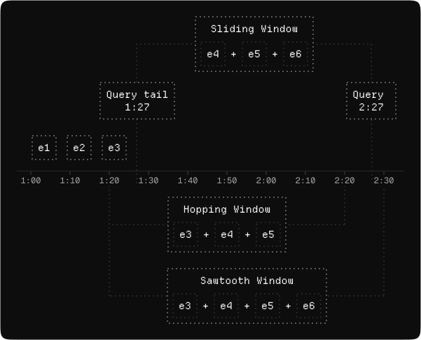
See the Realtime Event GroupBy examples for an example of windowed aggregations.
Bucketing
Expanding on the previous example - we now want to compute average purchase_price of a user_purchase source, but
bucketed by credit_card_type. So instead of producing a single double value, bucketing produces a map of credit_card_type to average_purchase_price.
Chronon can accept multiple bucket columns at once and Bucketing is specified as GroupBy.aggregations[i].buckets.
Bucketing always produces a map, and for online use-cases we require the bucket column to be a string. This requirement
comes from Chronon's usage of avro in the serving environment. We plan to remove this requirement at a later time.
Here's what the above example looks like modified to include buckets. Note that there are two primary changes:
- Include the selection of the
credit_card_typefield on the source (so that we have access to the field by which we want to bucket). - Specify the field as a bucket key in each aggregation that we want to apply it to.
See the Bucketed Example
Filtering
By default an aggregation consumes every row of the source. To aggregate only the rows matching a
condition, add a filter (a SQL boolean expression) and a column_alias to name the resulting
feature. For example, to count only the SMS sign-ups per device:
Aggregation(
    input_column="requestId",
    operation=Operation.COUNT,
    windows=[Window(1, TimeUnit.DAYS)],
    filter="intent = 'SMS'",       # only rows where this is true feed the aggregation
    column_alias="smsRequest",     # output feature -> smsRequest_count_1d
)filteris any SQL boolean expression over the source's columns; combine conditions withAND/OR/ parentheses.column_aliasreplacesinput_columnin the output name (<column_alias>_<op>_<window>) and is required wheneverfilteris set. It keeps names explicit, so one column can be aggregated under several filters without colliding.- The filter composes with
windowsandbuckets.
The same source column can back multiple filtered features:
aggregations=[
    Aggregation(input_column="phoneNumber", operation=Operation.COUNT, windows=[Window(1, TimeUnit.DAYS)],
                filter="status = 'failed'",  column_alias="failedPhoneNumber"),   # -> failedPhoneNumber_count_1d
    Aggregation(input_column="phoneNumber", operation=Operation.COUNT, windows=[Window(1, TimeUnit.DAYS)],
                filter="status = 'success'", column_alias="successPhoneNumber"),  # -> successPhoneNumber_count_1d
]
COUNTcounts non-null values ofinput_column, so a filteredCOUNTcounts rows where the predicate holds andinput_columnis non-null. To count all matching rows, pointCOUNTat a non-null column such as a key/id.
Conditional values with when / else
filter chooses which rows count. To compute what value to aggregate, use the when/else builder,
which renders a SQL CASE WHEN … END expression for use in a source's selects:
from ai.chronon.types import when

Query(selects={
    "adjusted_amount": when("region = 'US'", "amount * 1.1")
                       .when("region = 'EU'", "amount * 1.2")
                       .else_("amount"),
    # -> "CASE WHEN region = 'US' THEN amount * 1.1 WHEN region = 'EU' THEN amount * 1.2 ELSE amount END"
})
Chain .when(...) for more branches; .otherwise(...) aliases .else_(...). Omitting the else defaults to NULL. Values are raw SQL (a Python None renders as NULL; quote string literals yourself, e.g. "'SMS'").
Flattening
Chronon can extract values nested in containers and perform aggregations - over lists and maps. See details below for semantics.
Lists as inputs
Aggregations can also accept list columns as input. For example if we want average item_price from a user_purchase source, which contains item_prices as a list of values in each row - represented by a single credit card transaction.
Simply put, GroupBy.aggregations[i].input_column can refer to a column name which contains lists as values. In
traditional SQL this would require an expensive explode command and is supported natively in Chronon.
Maps as inputs
Aggregations over columns of type Map<String, Value>. For example - if you have two histograms this will allow for merging those
histograms using - min, max, avg, sum etc. You can merge maps of any scalar values types using aggregations that operate on scalar values.
The output of aggregations with scala values on map types is another map with aggregates as values.
Limitations:
- Map key needs to be string - because avro doesn't like it any other way.
- Map aggregations cannot be coupled with bucketing for now. We will add support later.
- Aggregations need to be time independent for now - will add support for timed version later.
NOTE: Windowing, Bucketing and Flattening can be flexibly mixed and matched.
Table of properties for aggregations
| aggregation | input type | nesting allowed? | output type | reversible | parameters | bounded memory |
|---|---|---|---|---|---|---|
| count | all types | list, map | long | yes | yes | |
| min, max | primitive types | list, map | input | no | yes | |
| top_k, bottom_k | primitive types | list, map | list<input,> | no | k | yes |
| unique_top_k | primitive & struct | list, map | list<input,> | no | k | yes |
| first, last | all types | NO | input | no | yes | |
| first_k, last_k | all types | NO | list<input,> | no | k | yes |
| average | numeric types | list, map | double | yes | yes | |
| variance, skew, kurtosis | numeric types | list, map | double | no | yes | |
| histogram | string | list, map | map<string, long> | yes | k=inf | no |
| approx_frequent_k | primitive types | list, map | map<string, long> | yes | k=inf | yes |
| approx_heavy_hitter_k | primitive types | list, map | map<string, long> | yes | k=inf | yes |
| approx_unique_count | primitive types | list, map | long | no | k=8 | yes |
| approx_percentile | primitive types | list, map | list<input,> | no | k=128, percentiles | yes |
| unique_count | primitive types | list, map | long | no | no |
Accuracy
accuracy is a toggle that can be supplied to GroupBy. It can be either SNAPSHOT or TEMPORAL. SNAPSHOT accuracy means that feature values are computed as of midnight only and refreshed once daily. TEMPORAL accuracy means that feature values are computed in realtime while serving, and in point-in-time-correct
fashion while backfilling.
When topic or mutationTopic is specified, we default to TEMPORAL otherwise SNAPSHOT.
This default is usually the desired behavior, so you rarely need to worry about setting this manually.
Online/Offline Toggle
online is a toggle to specify if the pipelines necessary to maintain feature views should be scheduled. This is for
online low-latency serving.
your_gb = GroupBy(
  ...,
  online=True
)
Note: Once a groupBy is marked online, the compiler
compile.pywill prevent you from updating it. This is so that you don't accidentally merge a change that release modified features out-of-band with model updates. You can overwrite this behavior by deleting the older compiled output. Our recommendation is to create a new versionyour_gb_v2instead.
Key Filter
key_filter is an optional EntitySource that limits which keys are written by the batch upload for an online GroupBy. It is useful when the aggregation source has many possible keys, but only a smaller active set should be
materialized in the online KV store. This only affects online batch uploads; it does not change the backfilled offline GroupBy table.
The filter is read from its snapshotTable at the upload date's partition. Chronon takes the distinct key tuples from
the filter source and semi-joins the aggregated upload rows against them after aggregation. The filter must be an entity
source with a snapshotTable, and its query.selects must produce columns named after at least one of the GroupBy keys. For multi-key GroupBys, the filter may select a subset of the keys and Chronon joins on the matching key
columns. If the filter produces no matching key columns, or no keys for that upload date, the upload fails instead of
writing an empty online snapshot.
active_users = Source(
    entities=EntitySource(
        snapshotTable="data.active_users",
        query=Query(
            selects=select("user_id"),
        ),
    )
)

user_purchases = GroupBy(
    sources=[purchase_events],
    keys=["user_id"],
    aggregations=[Aggregation(input_column="amount", operation=Operation.SUM)],
    online=True,
    key_filter=active_users,
)
Tuning
If you look at the parameters column in the above table - you will see k. k for top_k, bottom_k, first_k, last_k tells Chronon to collect k elements.
For unique_top_k - k tells Chronon to collect the top k unique elements ranked by their values.
For approx_unique_count and approx_percentile - k stands for the size of the sketch - the larger this is, the more
accurate and expensive to compute the results will be. Mapping between k and size for approx_unique_count is here for approx_percentile is the first table in here. percentiles for approx_percentile is an array of doubles between 0 and 1, where you want percentiles at. (Ex: "[0.25, 0.5, 0.75]")
For histogram - k keeps the elements with top-k counts. By default we keep everything.
Examples
The following examples are broken down by source type. We strongly suggest making sure you're using the correct source type for the feature that you want to express as a first step.
Realtime Event GroupBy examples
This example is based on the returns GroupBy from the quickstart guide that performs various aggregations over the refund_amt column over various windows.
source = Source(
    events=EventSource(
        table="data.returns", # This points to the log table with historical return events
        topic="events.returns",
        query=Query(
            selects=select("user_id","refund_amt"), # Select the fields we care about
            time_column="ts") # The event time
    ))

window_sizes = ["3d", "14d", "30d"] # Define some window sizes to use below

v1 = GroupBy(
    sources=[source],
    keys=["user_id"], # We are aggregating by user
    online=True,
    aggregations=[Aggregation(
            input_column="refund_amt",
            operation=Operation.SUM,
            windows=window_sizes
        ), # The sum of purchases prices in various windows
        Aggregation(
            input_column="refund_amt",
            operation=Operation.COUNT,
            windows=window_sizes
        ), # The count of purchases in various windows
        Aggregation(
            input_column="refund_amt",
            operation=Operation.AVERAGE,
            windows=window_sizes
        ),
        Aggregation(
            input_column="refund_amt",
            operation=Operation.LAST_K(2),
        ),
    ],
)
Bucketed GroupBy Example
In this example we take the Purchases GroupBy from the Quickstart tutorial and modify it to include buckets based on a hypothetical "credit_card_type" column.
source = Source(
    events=EventSource(
        table="data.purchases",
        query=Query(
            selects=select("user_id","purchase_price","credit_card_type"), # Now we also select the `credit card type` column
            time_column="ts")
    ))

window_sizes = ["3d", "14d", "30d"]

v1 = GroupBy(
    sources=[source],
    keys=["user_id"],
    online=True,
    aggregations=[Aggregation(
            input_column="purchase_price",
            operation=Operation.SUM,
            windows=window_sizes,
            buckets=["credit_card_type"] # Here we use the`credit_card_type` column as the bucket column
        ),
        Aggregation(
            input_column="purchase_price",
            operation=Operation.COUNT,
            windows=window_sizes,
            buckets=["credit_card_type"]
        ),
        Aggregation(
            input_column="purchase_price",
            operation=Operation.AVERAGE,
            windows=window_sizes,
            buckets=["credit_card_type"]
        ),
        Aggregation(
            input_column="purchase_price",
            operation=Operation.LAST_K(10),
            buckets=["credit_card_type"]
        ),
    ],
)
Simple Batch Event GroupBy examples
Example GroupBy with windowed aggregations. Taken from purchases.py.
Important things to note about this case relative to the streaming GroupBy:
- The default accuracy here is
SNAPSHOTmeaning that updates to the online KV store only happen in batch, and also backfills will be midnight accurate rather than intra day accurate. - As such, we do not need to provide a time column, midnight boundaries are used as the time along which feature values are updated. For example, a 30 day window computed using this GroupBy will get computed as of the prior midnight boundary for a requested timestamp, rather than the precise millisecond, for the purpose of online/offline consistency.
source = Source(
    events=EventSource(
        table="data.purchases", # This points to the log table with historical purchase events
        query=Query(
                selects=select("user_id","purchase_price"), # Select the fields we care about
            )
    ))

window_sizes = ["3d", "14d", "30d"] # Define some window sizes to use below

v1 = GroupBy(
    sources=[source],
    keys=["user_id"], # We are aggregating by user
    online=True,
    aggregations=[Aggregation(
            input_column="purchase_price",
            operation=Operation.SUM,
            windows=window_sizes
        ), # The sum of purchases prices in various windows
        Aggregation(
            input_column="purchase_price",
            operation=Operation.COUNT,
            windows=window_sizes
        ), # The count of purchases in various windows
        Aggregation(
            input_column="purchase_price",
            operation=Operation.AVERAGE,
            windows=window_sizes
        ), # The average purchases by user in various windows
        Aggregation(
            input_column="purchase_price",
            operation=Operation.LAST_K(10),
        ),
    ],
)
Batch Entity GroupBy examples
This is taken from the Users GroupBy from the quickstart tutorial.
"""
The primary key for this GroupBy is the same as the primary key of the source table. Therefore,
it doesn't perform any aggregation, but just extracts user fields as features.
"""

source = Source(
    entities=EntitySource(
        snapshotTable="data.users", # This points to a table that contains daily snapshots of the entire product catalog
        query=Query(
            selects=select("user_id","account_created_ds","email_verified"), # Select the fields we care about
        )
    ))

v1 = GroupBy(
    sources=[source],
    keys=["user_id"], # Primary key is the same as the primary key for the source table
    aggregations=None, # In this case, there are no aggregations or windows to define
    online=True,
)